PixeLens

Home Gravitational lensing

This is a program for reconstructing gravitational lenses from multiple-image data. It can explore ensembles of lens-models consistent with given data on several different lens systems at once.

You should see a button to the left saying Show PixeLens window. If not, try this help page.

Tutorial

Once PixeLens is up, you should see a GUI like this:

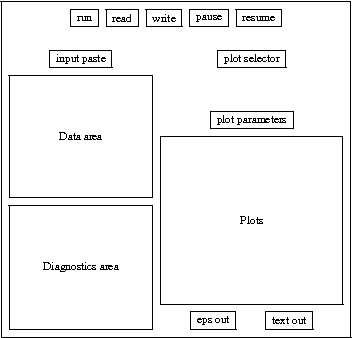
but some of the the buttons appear only in standalone mode.

You start by putting some data in the data area. The input paste button gives a number of suggestions you can paste in. (To edit the data area, the input choice must be set to edit.)

Now to make models press run. You can pause and resume as models are being generated.

The diagnostics area will track progress. (The standalone program also send some stuff to standard output---don't be alarmed by this, even if it says something fishy here.)

While models run in the background you can examine results in the plots. More about these later.

Running modes

The executable (or rather, Java byte code) and source code is in the PixeLens.jar file.

PixeLens is free software under the GNU GPL.

Running in a shell

You can execute the byte code from the command with
java -jar PixeLens.jar
or similar, or by some point-and-click method. This mode is more powerful, because it allows disk output.

Compiling from source code

You will need to need to install the Rambutan system. This is for preprocessing the literate Java format that all the code is written in into regular Java (and/or into TeX for annotated listings).

Command-line options

You can save the bother of pasting into the input area with
java -jar PixeLens.jar -i infile
On the other hand typing
java -jar PixeLens.jar -i infile -o outfile
bypasses the GUI. The ensemble gets written to outfile and diagnostics to standard output. This lets you run in batch mode and postprocess the results from the GUI later.

To change the number of threads (the default equals the number of shared-memory processors) use
java -jar PixeLens.jar --threads n

You can also pass command-line options directly to the JVM. There are many such options, but the only essential one is to increase the memory allocation. You can use
java -XmxnM -jar PixeLens.jar
where n is the maximum heapsize in Mb. The total memory required is a little under pixrad^4 kb for asymmetric models, and a quarter as much for symmetric models.

Input syntax

Input to PixeLens consists of model constants (redshifts, pixel size, and so on) and the image data. All input goes into the `Input area' of the GUI. It can be typed or pasted in, or read from a file. (By the way, line breaks in the input area count as spaces.)

Model constants

These are given by a keyword followed by one or two numbers.

Compulsory constants:

The input on each lens begins with
object nickname
The object name must be first, but the other model constants can appear in any order, before or after the image data.
For each lens, the radius of the mass map in pixels is set by
pixrad n
You can supply the lens redshift with zlens zl
or both redshifts with
redshifts zl zs
If the former, you must supply the source redshifts with the image data (see below). Also, if you use zlens the surface-density scale is the critical density for sources at infinity.

Optional constants:

For a symmetric mass map, put
symm
(default is asymmetric).
To set the radius of the mass map us
maprad r
where r is usually in arcsec. By default, the program will assign a maprad based on the image positions.
To allow external shear, use
shear angle
The angle is the approximate direction (relative to +x axis) of the group/cluster. The code will try directions within 45 deg of this.
The default is 100 models but you can change it with
models n
To fix the Hubble time, use
g value
where the value is in Gyr. If there are no time delays, fixing the Hubble time is compulsory; otherwise it is optional.
You can also provide
cosm Ω_m Ω_Λ
the default being (0.3,0.7).
To change the mininum steepness use
minsteep minval
The default is 0.5, meaning the mass profile is R^(-0.5) or steeper.
Similarly you can change the maximum steepness use
maxsteep maxval
If minval>maxval the program will silently ignore the latter.
You can fix the `annular density' (meaning the mean density in the annulus between the innermost and outermost images) with
kann value
This pins the shape degeneracy (but doesn't break it of course) and hence highlights shape degeneracies.

Image data

PixeLens recognizes two formats for image data.

In the single source-redshift format we write

double
x1 y1
x2 y2 dt2

quad
x1 y1
x2 y2 dt2
x3 y3 dt3
x4 y4 dt4

Here dt2 etc are time delays relative to the previous image (hence there is no dt1). Put 0 if the value is not measured. Meanwhile, the redshifts command must be used to supply both lens and source redshifts (see above).

If there are several source-redshifts, or the image system is not a double or quad, we need to write

multi n zs
x1 y1 p1
n-1 more such lines

Here zs is the source redshift, and p denotes the parity of an image: 1 for a minimum, 2 for a saddle point, 3 for a maximum. Meanwhile, the zlens command must be used.

The first format is more useful for galaxy lenses, the second more for cluster lenses.

You can have a mixture of doubles and quads in the first format, and of course you can mix image multiplicities in the second format. But you can't mix formats. (So if you want multiple source redshifts and time-delay measurements, you'll need to edit the source code!)

Important: The images must be in arrival-time order, even if the time delays are not known. Otherwise you will wrong results, or no solution.

Output formats

Figures

Use the plot selector to choose among several kinds of figure. Each plot also has parameters you can adjust. For example, the obj number (default 1) specifies which lens to plot stuff for.

If you are running in a shell, you can use the eps out and text out buttons for file output. The eps output is more or less what is shown on the GUI, but with better axis labels where needed. The eps files generated are simple enough to be easily edited by hand if required; for example you may want to change the colour scheme or add more annotation. The text output consists of tables of numbers (explained below) if there are interesting numbers to output; otherwise it just gives a blank file.

Pixellation

This draws the independent pixels, with images in red. The text output is a summary of various constants.

Mass

Mass contours in units of critical density are in green, reconstructed source(s) in cyan. You can change the contour step and/or zoom in/out. A negative contour step denotes logarithmic contours (the default of -2.512 corresponds to 1-mag contours). For asymmetric mass maps, you can also decompose into a symmetric (or `prim') residual (or `sec') parts.

The text output outputs the mass map as a table, followed by external shear if any.

Enclosed Mass

This shows circularly averaged mass profiles: choose between the enclosed mass and the surface-density profile. You can choose the confidence range for the error bars. Units are terasol for enclosed mass and terasol/kpc^2 for the surface density, against kpc.

The text output gives the same information in a table.

Arrival time

Contours in units of arcsec^2 for source number src, with the inferred source position in cyan. For step of 0.0 you get the saddle point contours.

If you choose a very small stepsize (of order 0.01 for galaxy lenses) you get an approximation to an Einstein ring.

Potential

For step of 0.0 you get the contours passing through each image. Use exag to exaggerate the shear part: exag=0 shows only the main lens potential, exag >> 1 shows only the shear.

Steepness

You can choose Hubble constant h against annular-density or h against radial index. The text output writes out the same information.

Time delays

Choose between histograms of the Hubble time or predicted time delays. Option of 0 shows the Hubble time, option of
2 1 2 4
shows time delay between images 2 and 4 of source 1 of lens 2, and so on. You can adjust the bin width. The text output gives the unbinned values.

Errors and warnings

No solution

The program runs and then stops.

Input area doesn't respond

To edit the input area, the input-paste selector must be set to `edit'. Editing is also disabled while the program is generating models, but re-enabled if you pause.

If you pause, then edit and then resume, the input area will revert without warning, i.e., it will discard your recent edits.

FAQ

Why use mass pixels rather than a potential grid?

In our first attempt at free-form lens models, we did indeed discretize the potential on a grid and defined the mass via a numerical second-derivative. Other non-parametric lens reconstruction programs also generally favor this route, which makes the equations simpler.

The problem is any numerical differentiation introduces noise. In particular, the implied mass distribution consist of delta functions, not necessarily all positive --- a far worse approximation than positive mass tiles as in PixeLens. To suppress such artifacts one would have to do more work, such as a spline interpolation or some ad-hoc regularization scheme.