
Fractals
This picture is generated using a mathematical formula - a fractal
Background
Using a home computer, Mandelbrot (1982) pioneered the mathematics of
fractals, a term which he coined in 1975. His fractals (the geometry of
fractional dimensions) helped describe or picture the actions of chaos, rather
than explain it.
The striking principle he discovered was that many of the irregular shapes that
make up the natural world, although seemingly random and chaotic in form, have a
simple organizing principle.
The biologist, Robert May, decided to see what would happen to the equation as
the growth rate value changes. At low values of the growth rate, the population
would settle down to a single number. For instance, if the growth rate value is
2.7, the population will settle down to .6292. As the growth rate increased, the
final population would increase as well. Then, something weird happened. As soon
as the growth rate passed 3, the line broke in two. Instead of settling down to
a single population, it would jump between two different populations. It would
be one value for one year, go to another value the next year, then repeat the
cycle forever. Raising the growth rate a little more caused it to jump between
four different values. As the parameter rose further, the line bifurcated
(doubled) again. The bifurcations came faster and faster until suddenly, chaos
appeared. Past a certain growth rate, it becomes impossible to predict the
behaviour of the equation. However, upon closer inspection, it is possible to
see white strips. Looking closer at these strips reveals little windows of
order, where the equation goes through the bifurcations again before returning
to chaos. This self-similarity, the fact that the graph has an exact copy of
itself hidden deep inside, came to be an important aspect of chaos.
An employee of IBM, Benoit Mandelbrot was a mathematician studying this
self-similarity. One of the areas he was studying was cotton price fluctuations.
No matter how the data on cotton prices was analyzed, the results did not fit
the normal distribution. Mandelbrot eventually obtained all of the available
data on cotton prices, dating back to 1900. When he analyzed the data with IBM's
computers, he noticed an astonishing fact:
The numbers that produced aberrations from the point of view of normal
distribution produced symmetry from the point of view of scaling. Each
particular price change was random and unpredictable. But the sequence of
changes was independent on scale: curves for daily price changes and monthly
price changes matched perfectly. Incredibly, analysed Mandelbrot's way, the
degree of variation had remained constant over a tumultuous sixty-year period
that saw two World Wars and a depression.
Mandelbrot analyzed not only cotton prices, but many other phenomena as well. At
one point, he was wondering about the length of a coastline. A map of a
coastline will show many bays. However, measuring the length of a coastline off
a map will miss minor bays that were too small to show on the map. Likewise,
walking along the coastline misses microscopic bays in between grains of sand.
No matter how much a coastline is magnified, there will be more bays visible if
it is magnified more.
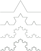
Helge von Koch, captured this idea in a mathematical
construction called the Koch curve (1906). To create a Koch curve, imagine an
equilateral triangle. To the middle third of each side, add another equilateral
triangle. Keep on adding new triangles to the middle part of each side, and the
result is a Koch curve. (See figure below) A magnification of the Koch curve looks
exactly the same as the original. It is another self-similar figure.
The Koch curve brings up an interesting paradox. Each time new triangles are
added to the figure, the length of the line gets longer. However, the inner area
of the Koch curve remains less than the area of a circle drawn around the
original triangle. Essentially, it is a line of infinite length surrounding a
finite area!
To get around this difficulty, mathematicians invented fractal dimensions.
Fractal comes from the word fractional. The fractal dimension of the Koch curve
is somewhere around 1.26. A fractional dimension is impossible to conceive, but
it does make sense. The Koch curve is rougher than a smooth curve or line, which
has one dimension. Since it is rougher and more crinkly, it is better at taking
up space. However, it's not as good at filling up space as a square with two
dimensions is, since it doesn't really have any area. So it makes sense that the
dimension of the Koch curve is somewhere in between the two.
Fractal has come to mean any image that displays the attribute of
self-similarity. The bifurcation diagram of the population equation is fractal.
The Lorenz Attractor is fractal. The Koch curve is fractal.
During this time, scientists found it very difficult to get work published about
chaos. Since they had not yet shown the relevance to real-world situations, most
scientists did not think the results of experiments in chaos were important. As
a result, even though chaos is a mathematical phenomenon, most of the research
into chaos was done by people in other areas, such as meteorology and ecology.
The field of chaos sprouted up as a hobby for scientists working on problems
that maybe had something to do with it.
Later, a scientist by the name of Feigenbaum was looking at the bifurcation
diagram again. He was looking at how fast the bifurcations come. He discovered
that they come at a constant rate. He calculated it as 4.669. In other words, he
discovered the exact scale at which it was self-similar. Make the diagram 4.669
times smaller, and it looks like the next region of bifurcations. He decided to
look at other equations to see if it was possible to determine a scaling factor
for them as well. Much to his surprise, the scaling factor was exactly the same.
Not only was this complicated equation displaying regularity, the regularity was
exactly the same as a much simpler equation. He tried many other functions, and
they all produced the same scaling factor, 4.669.
This was a revolutionary discovery. He had found that a whole class of
mathematical functions behaved in the same, predictable way. This universality
would help other scientists easily analyze chaotic equations. Universality gave
scientists the first tools to analyze a chaotic system. Now they could use a
simple equation to predict the outcome of a more complex equation.
Many scientists were exploring equations that created fractal equations. The
most famous fractal image is also one of the most simple. It is known as the
Mandelbrot set (pictures of the Mandelbrot set). The equation is simple: z=z2+c.
To see if a point is part of the Mandelbrot set, just take a complex number z.
Square it, then add the original number. Square the result, then add the
original number. Repeat that ad infinitum, and if the number keeps on going up
to infinity, it is not part of the Mandelbrot set. If it stays down below a
certain level, it is part of the Mandelbrot set. The Mandelbrot set is the
innermost section of the picture, and each different shade of grey represents
how far out that particular point is. One interesting feature of the Mandelbrot
set is that the circular humps match up to the bifurcation graph. The Mandelbrot
fractal has the same self-similarity seen in the other equations. In fact,
zooming in deep enough on a Mandelbrot fractal will eventually reveal an exact
replica of the Mandelbrot set, perfect in every detail.
Look again at our original mapping:
f(x) --> x2 + c.
The graph of this function is a parabola when "x" and "c" are real numbers. The orbits of well-behaved seeds are bounded for parameter values in the interval [-2, 1/4]. These orbits can settle on to attracting fixed points, be periodic, or ergodic. A small set of fixed points, the repelling fixed points, do not generate orbits in the traditional sense. They neither roam nor run off to infinity and one need not wait for them to exhibit "characteristic" behaviour. They are permanently and immutably fixed and nearby points avoid them. They lie on the frontier between those seeds with bounded orbits and those with unbounded orbits. Such is the behaviour in general for all points and all parameter values; or is it? The discussion so far has been constrained by a prejudice for real numbers. What happens when we admit that i = sqrt(-1) has a solution? How does our function behave when "z" and "c" are complex numbers? The answer, of course, is the same but the results are much more interesting than such a flip statement implies.
The map
f(z) --> z2 + c
is equivalent to the two-dimensional map
f(x, y) --> (x2 - y2 + a, 2xy + b)
where z = x + iy = (x, y) is a point to be iterated and c = a + ib = (a, b) acts as the parameter. Thus, the quadratic map of the complex numbers can be studied as a family of transformations to the complex plane.
 |
 |
 |
| Stretch points inside the unit circle towards the origin. Stretch points outside towards infinity. | Wrap the plane around itself once without cutting or tearing such that every every angle value has doubled. | Shift the plane over so the origin lies on (a, b). |
Actually, it's easier to discuss these transformations if we represent the complex numbers as points on a complex sphere. The origin would be one pole and infinity another pole with the unit sphere being the equator. Imagine placing a light bulb at the infinity pole. Points on the sphere would leave shadows in unique positions on the plane. The complex plane is thus a projection of the complex sphere. While this is easier to deal with because we have a single point called infinity, it is not easier to diagram. Let's give it a shot.
Stereographic Projection of the Complex Sphere on to the
Complex Plane

 |
 |
 |
| Stretch points below the unit equator towards the origin pole. Stretch points above the equator towards the infinity pole. | Wrap the sphere around itself once without cutting or tearing such that every longitude value has doubled. | Stretch the sphere so the origin pole shifts to the point (a, b) but the infinity pole stays fixed. |
This family of mappings is said to be conformal; that is, it leaves angles unchanged. Despite all this stretching, twisting, and shifting there is always a set of points that transforms into itself. Such sets are called the Julia sets after the French mathematician Gaston Julia who first conceived of them in the 1910s. The special case of c = (0, 0) has already been dealt with (the set is the unit circle). Let's look at a variety of parameter values and see what kind of Julia sets arise. Some examples are shown below.
 |
 |
 |
 |
| c = 0.275 | c = 1/4 | c = 0 | c = -3/4 |
 |
 |
 |
 |
| c = -1.312 | c = -1.375 | c = -2 | c = i |
 |
 |
 |
 |
| c = (+0.285, +0.535) | c = (-0.125, +0.750) | c = (-0.500, +0.563) | c = (-0.687, +0.312) |
Sets on the real axis are reflection symmetric while those with complex parameter values show rotational symmetry. With the exception of the parameter value c = 0, all Julia sets exhibit self-similarity. There are two broad categories of Julia sets: those which are connected and those which are not. Of the twelve examples shown, only the first and last are disconnected. The distinction between the two categories is extreme. Disconnected sets are completely disconnected into a countably infinite assembly of isolated points. In addition, these points are arranged in dense groups such that any finite disk surrounding a point contains at least one other point in the set. Such sets are said to be dustlike. As they can be shown to be similar to the Cantor middle thirds set, they are often called Cantor dusts. In contrast, the connected sets are completely connected. Topologically, they are either equivalent to a severely deformed circle or to a line with an infinite series of branches and sub-branches called a dendrite (at c = i for example).
The factor that determines whether a Julia set is wholly connected or wholly disconnected is the parameter value. Thus it would be instructive to plot the behaviour of the Julia sets for all parameter values. The resulting construction would be the complex analogue of a bifurcation drawing. At first glance, this seems a daunting task. Plotting every possible Julia set and then examining it to determine whether it was connected or not would take an eternity. Luckily for us, however, we need only study the behaviour of one point in the complex plane. Given a family of complex iterative maps, the set of all parameter values that produce wholly connected Julia sets is determined by the behaviour of a single seed value: the origin. If the orbit of the origin never escapes to infinity then it is either a part of the set or it is trapped inside it. If the origin is a part of the set, the set is dendritic. If it is trapped inside the set, the set is topologically equivalent to a circle and thus is wholly connected. This trick was discovered by the Polish-American mathematician Benoit Mandelbrot and in his honour the set of all parameter values whose Julia sets are wholly connected is called a Mandelbrot set. The Mandelbrot set for the quadratic mapping f: z --> z2 = c is shown below for all parameters c = x = iy in the range x = [-2, 1/2] y = [-2, 2]. Some wholly connected Julia sets were also added and their approximate location in parameter space indicated. This type of arrangement is known as a constellation diagram.
A Mandelbrot Set with 8 Accompanying Julia Sets in a
Constellation Diagram
Click on the image to see a very, very large copy (1729 x 1588).

Note the similarities between any Julia set and the corresponding parameter space region on the Mandelbrot set. The Julia sets that are pinched vertically are found where the Mandelbrot set is pinched vertically. Likewise the set which is pinched horizontally is found on the extreme right side in a region that is pinched horizontally. The dendrite corresponds to a parameter point on a filament at the top and the long tail to the left produces a Julia set that is similarly long and tail-like. Such similarities are found at the microscopic level as well. Not only does the Mandelbrot set tell whether a corresponding Julia set is connected or disconnected, it also suggests its appearance.
An interesting way to see the variety of Julia sets is by means of a cascade.
The main body of the Mandelbrot set is a cardioid with a series of successively smaller circles attached to it in a chain running along the x-axis in the negative direction. The attachment points on this chain correspond to the bifurcation points of the simple one-dimensional iterative map. Thus, each circle on the x-axis corresponds to a region of differing periodicity. The ratio of the diameters of successive circles approaches Feigenbaum's constant "delta". Note too, how the long tail-like region is punctuated with little islands. This corresponds to the chaotic regime and the islands to the odd period windows. Recall how in the one-dimensional case the structure of the windows was similar to the overall bifurcation diagram. Likewise these windows are miniature mutated copies of the whole Mandelbrot set. This structure also repeats itself radially around the set. Each major bulb has smaller bulbs budding off it which in turn have bulbs attached to them and so on. The whole set is bristling with filaments, each with its own array of window-like, mutated copies of the whole set. The Mandelbrot set is a wholly connected archipelago of self-similar islets linked by an array of extremely twisty, ever branching fibers. There is no end to the detail present in the Mandelbrot set as the following set of successive magnifications show.
 |
 |
 |
 |
| M = 10-1 | M = 100 | M = 101 | M = 102 |
 |
 |
 |
 |
| M = 103 | M = 104 | M = 105 | M = 106 |
 |
 |
 |
 |
| M = 107 | M = 108 | M = 109 | M = 1010 |
 |
 |
 |
 |
| M = 1011 | M = 1012 | M = 1013 | M = 1014 |
The diagrams below give some idea of the variety of structures that can be found in the Mandelbrot set. The first row of diagrams show some of the decorations attached to the bulbs surrounding the bays. Note how the branching patterns are similar to each other, yet still unique. (Incidentally, the number of branches equals the period of the points within a particular bulb.) The second row of diagrams show some of the "mini-mandelbrots" that crop up along the filaments. Each is unique, but yet still unmistakably a Mandelbrot set in appearance. These pictures illustrate an important characteristic of the Mandelbrot set. Whereas fragments of a Julia set are strictly similar to the set as a whole, fragments of the Mandelbrot are only quasi-similar to the set as a whole. Furthermore, the motif of this quasi-self-similarity varies from one region to another and from one level of magnification to another.
 |
 |
 |
 |
| Period 3 Bulb | Period 4 Bulb | Period 5 Bulb | Period 7 Bulb |
 |
 |
 |
 |
| Mini-Mandelbrot | Mini-Mandelbrot | Mini-Mandelbrot | Mini-Mandelbrot |
 |
 |
 |
 |
| c = (-0.747..., +0.108...) | c = (-0.760..., +0.081...) | c = (-1.265..., +0.046...) | c = (+0.349..., +0.357...) |
 |
 |
 |
 |
| c = (-0.154..., +1.031...) | c = (-0.154..., +1.031...) | c = (-0.154..., +1.031...) | c = (-0.154..., +1.031...) |
One way to picture Mandelbrot and Julia sets is as complex ordered pairs (c, z) such that the mapping f: z --> z2 + c does not escape to infinity when iterated. Julia sets are slices parallel to the z-axis while the Mandelbrot set is a slice along the c-axis through the origin. As the coordinate system is complex, however, these "axes" are actually planes. The Mandelbrot and Julia sets are therefore two-dimensional cross sections through a four-dimensional parent set; the mother of all iterated quadratic mappings so to speak.
The exotic sets shown in the following movie are successive slices through the four-dimensional mother set as we shift the cross sectional plane from the z = 0 plane of the Mandelbrot set to the c = -1 plane of a particular Julia set (the San Marco Dragon).
In this chapter, I have touched on some of the topics arising out of the study of iterated mappings, expanding the simple one-dimensional case to the multi-dimensional and complex realms. By extension, one can imagine other related systems worthy of an equal amount of study. We have not addressed the analysis of other iterated mappings on the complex plane: higher powers such as "z4 + c" or "z6 + c"; trigonometric functions like "cos z + c"; hyperbolic or exponential functions, and so on. We also have not dealt with functions driven by periodic or random fluctuations, nor those with discontinuities and corners. And if we allow complex numbers, we must also allow quaternions, octernions and the rest of their higher dimensional cousins. Not surprisingly, someone has already done most of this.
By definition, the null set (![]() )
and only the null set shall have the dimension -1. The dimension on any other
space will be defined as one greater that the dimension of the object that could
be used to completely separate any part of the first space from the rest. It
takes nothing to separate one part of a countable set from the rest of the set.
Since nothing (
)
and only the null set shall have the dimension -1. The dimension on any other
space will be defined as one greater that the dimension of the object that could
be used to completely separate any part of the first space from the rest. It
takes nothing to separate one part of a countable set from the rest of the set.
Since nothing (![]() )
has dimension -1, any countable set has a dimension of 0 (-1 + 1 = 0). Likewise,
a line has dimension 1 since it can be separated by a point (0 + 1 = 1), a plane
has dimension 2 since it can be separated by a line (1 + 1 = 2), and a volume
has dimension 3 since it can be separated by a plane (2 + 1 = 3). We have to
modify this dimension a little bit, however.
)
has dimension -1, any countable set has a dimension of 0 (-1 + 1 = 0). Likewise,
a line has dimension 1 since it can be separated by a point (0 + 1 = 1), a plane
has dimension 2 since it can be separated by a line (1 + 1 = 2), and a volume
has dimension 3 since it can be separated by a plane (2 + 1 = 3). We have to
modify this dimension a little bit, however.
Sure a countable set can be separated by nothing, but it can also be separated by another countable set or a line or a plane. Take the rational numbers, for example. They form a countable infinite set. By embedding the set in the real number line, we could separate one point from any other with an irrational number. This set is has dimension 0, which would give the rational numbers a dimension of 1 (0 + 1 = 1). By embedding the set in the coordinate plane, we could also use any line with an x-intercept. This would give the rational numbers a dimension of 2 (1 + 1 = 2). We could also use planes if we embedded the set in a euclidean three-space and so on. I think it would be all right if we used the minimum value and called it the dimension of the space.
What about our composite spaces (![]() )
and (
)
and (![]()
![]() )?
We want the first to have dimension 1 and the second dimension 2. The x-shaped
space is no problem. The least dimensional entity needed to separate it would be
a point even at the intersection. The point and filled square is a bit more
challenging. We need to distinguish between local
dimension and global dimension. If we use
the last definition and apply it to the set as a whole, then the space (
)?
We want the first to have dimension 1 and the second dimension 2. The x-shaped
space is no problem. The least dimensional entity needed to separate it would be
a point even at the intersection. The point and filled square is a bit more
challenging. We need to distinguish between local
dimension and global dimension. If we use
the last definition and apply it to the set as a whole, then the space (![]()
![]() )
would have dimension 0. If on the other hand, we examine it region by region we
find that the point part has dimension 0 while any part of the square region has
dimension 2. This is an example of a local dimension. The global dimension of
the whole space should be two-dimensional so we need to modify our definition
slightly. The dimension of a space should be the maximum of its local dimensions
where the local dimension is defined as one more than the dimension of the
lowest dimensional object with the capacity to separate any neighborhood of the
space into two parts.
)
would have dimension 0. If on the other hand, we examine it region by region we
find that the point part has dimension 0 while any part of the square region has
dimension 2. This is an example of a local dimension. The global dimension of
the whole space should be two-dimensional so we need to modify our definition
slightly. The dimension of a space should be the maximum of its local dimensions
where the local dimension is defined as one more than the dimension of the
lowest dimensional object with the capacity to separate any neighborhood of the
space into two parts.
The measure defined above is called the topological dimension of a space. A topological property of an entity is one that remains invariant under continuous, one-to-one transformations or homeomorphisms. A homeomorphism can best be envisioned as the smooth deformation of one space into another without tearing, puncturing, or welding it. Throughout such processes, the topological dimension does not change. A sphere is topologically equivalent to a cube since one can be deformed into the other in such a manner. Similarly, a line segment can be pinched and stretched repeatedly until it has lost all its straightness, but it will still have a topological dimension of 1. Take the example below.
The result the is the Koch coastline, which evolves something like this.
The Koch Coastline
![]()
With each iteration the curve length increases by the factor 4/3. The infinite repeat of this procedure sends the length off to infinity. The area under the curve, on the other hand, is given by the series
1+ (4/9) + (4/9)2 + (4/9)3 + ...
which converges to 9/5 (assuming the area under the first curve is 1). These results are unusual but not disturbing. Such is not the case for the next curve.
The result is something like the diagrams below. (Cell lines were omitted in the third iteration for clarity. The last diagram represents the hypothetical result of an infinite iteration.)
Peano Monster Curve (A Variation on Hilbert's Version)

This curve twists so much that it has infinite length. More remarkable is that it will ultimately visit every point in the unit square. Thus, there exists a continuous, one-to-one mapping from the points in the unit interval to the points in the unit plane. In other words, an object with topological dimension one can be transformed into an object with topological dimension two through a procedure that should not allow for such an occurrence. Simple bending and stretching should leave the topological dimension unchanged, however. This is a Peano monster curve (actually, a variation on Hilbert's version of Peano's original), so called because of its monstrous or pathological nature. Since there are no such things as monsters, we have nothing to fear. The Koch and Peano curves raise questions about the meaning of dimension that will be answered in the next section.
There really was a reason to fear pathological entities like the Koch coastline and Peano's monster curve. Here were creations so twisted and distorted that they did not fit into the box of contemporary mathematics. Luckily, mathematics was fortified by the study of the monsters and not destroyed by them. Whatever doesn't kill you only makes you stronger.
Take the Koch coastline and examine it through a badly focused lens. It appears to have a certain length. Let's call it 1 unit. Sharpen the focus a bit so that you can resolve details that are 1/3 as big as those seen with the first approximation. The curve is now four times longer or 4 units. Double the resolution by the same factor. Using a focus that reveals details 1/9 the first focus gives us a coastline 16 times longer and so on. Such an activity hints at the existence of a quantifiable characteristic.
To be a bit more precise, every space that feels "real" has associated with it a sense of distance between any two points. On a line segment like the Koch coastline, we arbitrarily chose the length of one side of the first iterate as a unit length. On the Euclidean coordinate plane the distance between any two points is given by the Pythagorean theorem
s2 = x2 + y2.
In relativity, the "distance" between any two events in space-time is given by the proper time
s2 = c2t2 - x2 - y2 - z2.
Such distance establishing relationships are called metrics and a space that has a metric associated with it is called a metric space. One of the more famous, non-euclidean metrics is the Manhattan metric (or taxicab metric). How far is the corner of 33rd and 1st from 69th and 5th? Answer: 36 blocks and 4 avenues or 40 units. (We have to bend reality a bit and assume that city blocks in Manhattan are square and not rectangular.) Metrics are also used to create neighborhoods in a space. Pick a point in a metric space. This point plus all others lying less than or equal to a certain distance away comprise a region of the space called a closed disk. The term disk is used because such regions are disk-shaped in the coordinate plane with the usual metric but any shape is possible. In euclidean three-space disks would be balls while in a two-space with a Manhattan metric they would be squares.
How many disks does it take to cover the Koch coastline? Well, it depends on their size of course. 1 disk with diameter 1 is sufficient to cover the whole thing, 4 disks with diameter 1/3, 16 disks with diameter 1/9, 64 disks with diameter 1/27, and so on. In general, it takes 4n disks of radius (1/3)n to cover the Koch coastline. If we apply this procedure to any entity in any metric space we can define a quantity that is the equivalent of a dimension. The Hausdorff-Besicovitch dimension of an object in a metric space is given by the formula
![]()
where N(h) is the number of disks of size h needed to cover the object. Thus the Koch coastline has a Hausdorff-Besicovitch dimension which is the limit of the sequence
![]()
Is this really a dimension? Apply the procedure to the unit line segment. It takes 1 disk of diameter 1, 2 disks of diameter 1/2, 4 disks of diameter 1/4, and so on to cover the unit line segment. In the limit we find a dimension of
![]()
This agrees with the topological dimension of the space.
The problem now is, how do we interpret a result like 1.261859507...? This does not agree with the topological dimension of 1 but neither is it 2. The Koch coastline is somewhere between a line and a plane. Its dimension is not a whole number but a fraction. It is a fractal. Actually fractals can have whole number dimensions so this is a bit of a misnomer. A better definition is that a fractal is any entity whose Hausdorff-Besicovitch dimension strictly exceeds its topological dimension (D > DT). Thus, the Peano space-filling curve is also a fractal as we would expect it to be. Even though its Hausdorff-Besicovitch dimension is a whole number (D = 2) its topological dimension (DT = 1) is strictly less than this. The monster has been tamed. It should be possible to use analytic methods like those described above on all sorts of fractal objects. Whether this is convenient or simple is another matter. Fractals produced by simple iterative scaling procedures like the Koch coastline are very easy to handle analytically. Julia and Mandelbrot sets, fractals produced by the iterated mapping of continuous complex functions, are another matter. There's no obvious fractal structure to the quadratic mapping, no hint that a "monster" curve lurks inside, and no simple way to extract an exact fractal dimension. If there are analytic techniques for calculating the fractal dimension of an arbitrary Julia set they are well hidden. A narrow and quick search of the popular literature reveals nothing on the ease or impossibility of this task. There are, however, experimental techniques. Take any plane geometric object of finite extent (fractal or otherwise) and cover it with a single closed disk. Any type of disk will do, so to make life easy we will use a square; the disk of the Manhattan metric in the plane. Record its dimension and call it "h". Repeat the procedure with a smaller box. Record its dimension and the number of boxes "N(h)" required to cover the object. Repeat with ever smaller boxes until you have reached the limit of your resolving power as shown in the figure to the right. Plot the results on a graph with "log N(h)" on the vertical axis and "log (1/h)" on the horizontal axis. The slope of the best fit line of the data will be an approximation of the Hausdorff-Besicovitch dimension of the object. The following are the results of a few sample experiments using this box-counting method. I think with a bit of refinement, the deviations could all be brought below 5%. |
| Koch Coastline |
dimension (experimental) = 1.18 dimension (analytical) = 1.26 deviation = 6% |
||||||||||||||||||||||||||
|
 |
||||||||||||||||||||||||||
San Marco Dragon |
dimension (experimental) = 1.16 dimension (analytical) = ?? deviation = ?? |
||||||||||||||||||||||||||
|
 |
||||||||||||||||||||||||||
Rectangle |
dimension (experimental) = 1.82 dimension (analytical) = 2.00 deviation = 9% |
||||||||||||||||||||||||||
|
 |
||||||||||||||||||||||||||
Tree Silhouette |
dimension (experimental) = 1.73 dimension (analytical) = ?? deviation = ?? |
||||||||||||||||||||||||||
|
 |
