
Chaos
History
In 1890's Poincare entered a contest formulated by the King of Sweden in which one of the questions was to show the solar system as modelled by Newtons equations is dynamically stable. The question was nothing more than a generalization of the famous three body problem, which was considered one of the most difficult problems in mathematical physics.
In essence, the three body problem consists of nine simultaneous differential equations. The difficulty was in showing that a solution in terms of invariants converges. While Poincaré did not succeed in giving a complete solution, his work was so impressive that he was awarded the prize anyway.
"If we knew exactly the laws of nature and the situation of the universe at the initial moment, we could predict exactly the situation of that same universe at a succeeding moment. but even if it were the case that the natural laws had no longer any secret for us, we could still only know the initial situation approximately. If that enabled us to predict the succeeding situation with the same approximation, that is all we require, and we should say that the phenomenon had been predicted, that it is governed by laws. But it is not always so; it may happen that small differences in the initial conditions produce very great ones in the final phenomena. A small error in the former will produce an enormous error in the latter. Prediction becomes impossible, and we have the fortuitous phenomenon." - in a 1903 essay "Science and Method"
However, the discovery of chaos is credited to Edward Lorenz, who in 1960 was carrying out computer modelling of weather. He wanted to look at a particular sequence again and to save time, he started in the middle of the sequence, instead of the beginning. He entered the number off his last printout and left to let it run. When he came back an hour later, the sequence had evolved differently. Instead of the same pattern as before, it diverged from the pattern, ending up wildly different from the original.
Eventually he figured out what happened. The computer stored the numbers to six decimal places in its memory. To save paper, he only had it print out three decimal places. In the original sequence, the number was .506127, and he had only typed the first three digits, .506.
This phenomenon, common to chaos theory, is also known as sensitive dependence on initial conditions. Just a small change in the initial conditions can drastically change the long-term behaviour of a system. Such a small amount of difference in a measurement might be considered experimental noise, background noise, or an inaccuracy of the equipment. Such things are impossible to avoid in even the most isolated lab. With a starting number of 2, the final result can be entirely different from the same system with a starting value of 2.00000000000000000000000001. It is simply impossible to achieve this level of accuracy - just try and measure something to the nearest millionth of an inch!
From this idea, Lorenz stated that it is impossible to predict the weather accurately. However, this discovery led Lorenz on to other aspects of what eventually came to be known as chaos theory.
The Lorenz Attractor
Determinism implies predictability only in the idealised limit of infinite precision. In the case of a simple pendulum, for example, the behaviour will be determined uniquely by the initial conditions. The initial data includes the position of the bob, so exact predictability demands that we must assign the real number to the position that correctly describes the distance of the pendulums centre from a fixed point and this infinite precision is impossible.
A deterministic system is one in which future states are completely determined, through some dynamical law, by preceding states. Brownian motion appears random and non-deterministic simply because of our inability to calculate all of the molecular collisions that take place. Given enough information, Brownian motion is predictable and deterministic. A double pendulum may seem to follow very simple laws of physics and should be deterministic, but in fact the future motion can not be predicted. This is the origin of deterministic chaos.
Recall the discussion on entropy and predictability. Given the positions and velocities of all the air molecules in a box it is possible to predict the past and future state. But this requires arbitrarily high precision in the initial conditions and our trajectory calculations.
The laws of thermodynamics bypass this lack of ability and knowledge by coming up with laws that govern the global properties of systems. However these laws do not help if the application is a complex dynamical system.
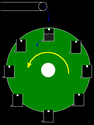
Lorenz started to look for a simpler system that had sensitive dependence on initial conditions. His first discovery had twelve equations, and he wanted a much more simple version that still had this attribute. He took the equations for convection, and stripped them down, making them unrealistically simple. The system no longer had anything to do with the convection, but it did have sensitive dependence on its initial conditions, and there were only three equations this time. Later, it was discovered that his equations precisely described a water wheel - basically the Navier-Stokes equations:


Mathematicians have known about nonlinearity (a characteristic of discontinuous events) since, the work of Henri Poincaré, at the turn of this century. Nonlinear equations have been around for a long time, but no one was able to solve them, and traditional scientists and engineers simply ignored all nonlinear portions of their calculations. Most equations that attempt to predict the actions of nature or natural materials are close approximations rather than exact. They contain one or more factors of nonlinearity; which are approximated by using constants called fudge factors!
In 1971, David Ruelle and Floris Takens described a phenomena they called a
strange attractor (a special type of attractor today called a chaotic
attractor). This strange phenomena was said to reside in what they called phase
space (a geometric depiction of the state space of a system) and a whole new
element of chaos theory was born. Phase space allows scientists to map
information from complex systems, make a picture of their moving parts, and
allows insight into a dynamic system's possibilities.
Ruelle's association of turbulence with a strange attractor was so
revolutionary, he was not able to publish his paper, and finally published it
himself. He writes, “Actually, I was an editor of the journal, and I accepted
the paper for publication. This is not a recommended procedure in general, but I
felt that it was justified in this particular case”.
Another pioneer of the new science was Mitchell Feigenbaum. His work, in the
late 1970s, was so revolutionary that several of his first manuscripts were
rejected for publication because they were so novel they were considered
irreverent (Gleick, 1987). He discovered order in disorder. He looked deeply
into turbulence, the home of strange attractors, and saw universality. He
developed a method to measure turbulence and found a structure embedded in
nonlinear systems.
Feigenbaum showed that period doubling is the normal way that order breaks down
into chaos. He calculated universal numbers which represent ratios in the scale
of transition points that occur during the process of period doubling. These
ratios are now called Feigenbaum numbers. Gleick (1987) mentions that Richard J.
Cohen, and his medical colleagues at MIT, found that period doubling is
associated with the onset of a heart attack. This finding brought chaos science
into the domain of medical science. Chaos is applied to numerous different
disciplines, from engineering to communication.
Perhaps the
most startling finding to come out of this new scientific theory is that order
exists within chaos. In fact, order comes from chaotic conditions.
Resonances
Forced resonances can lead to interesting consequences - look at the Tacoma bridge in Washington...
(Washington state lost three bridges due to engineering problems - the I90 floating bridge sank in 1990!)

Hamiltonian Chaos
Double pendulum with Poincare section
Iteration
One of the great breakthroughs in mathematics in this century has been the realization that even the simplest of dynamical systems may behave extremely unpredictably. Take the real functions
y = x2 + c and x = y
equations for a parabola and straight line respectively. There are few equations simpler than these and yet from them we can generate some rather complex and interesting behaviour.
One way to interpret the functions is as two curves in the plane. A second way is as a series of instructions.
The first two instructions together form a mapping of one number on to another:
f(x') --> x2 + c.
The addition of the third step results in an iterated mapping. We will use the symbol fn(x) to represent the nth iterate of our original value "x". The instructions tell us to generate a series of numbers
x, f(x), f2(x), f3(x),... , fn(x),...
which we will call the orbit. The initial value "x" is called the seed of the orbit. Note that there is no instruction telling us when to stop. Thankfully, humans are not quite so stupid as are the instructions given to them. Somewhere in this sequence, a pattern will emerge that will allow us to stop iterating and make a judgment. If it takes us too long to arrive at a decision or if we just get tired of doing all the work we can always turn it over to a computer. Let us now look at the behaviour of some orbits.
The parameter c = 0 is by far the easiest to deal with as
f(x') --> x2 + c
will yield the following results:
![]()
All orbits approach either zero or infinity except for those with seed x = +/-1. The points zero and infinity are called attracting fixed points or sinks because they attract the orbits of the points around them while +/-1 are called repelling fixed points or sources for the opposite reason.
When c > 1/4 the parabola is entirely above the diagonal line and all seed values will be driven off to infinity. When c = 1/4 the parabola and the diagonal line intersect at 1/2. Seeds with absolute value greater than 1/2 will expand off to infinity while those in the interval 0 <= |x| <= 1/2 approach 1/2 asymptotically. After about 700 iterations these seeds will have reached 4.99. The results of the first ten iterations for some seed values are presented in the table below.
| ±1 | ±0.75 | ±0.5 | ±0.25 | ±0.1 | 0 |
|---|---|---|---|---|---|
| +1.25 | +0.812 | +0.5 | +0.3125 | +0.26 | +0.25 |
| +1.812 | +0.910 | +0.5 | +0.3476562 | +0.3176 | +0.3125 |
| +3.535 | +1.078 | +0.5 | +0.3708648 | +0.3508697 | +0.3476562 |
| +12.747 | +1.412 | +0.5 | +0.3875407 | +0.3731096 | +0.9708648 |
| +162.744 | +2.246 | +0.5 | +0.4001878 | +0.3892107 | +0.3875407 |
| +26485.994 | +5.296 | +0.5 | +0.4101503 | +0.4014850 | +0.4001878 |
| +701507907 | +28.297 | +0.5 | +0.4182232 | +0.4111902 | +0.4101503 |
| +4.921e+17 | +800.985 | +0.5 | +0.4249107 | +0.4190774 | +0.4182232 |
| +2.421e+35 | +64158.262 | +0.5 | +0.4305491 | +0.4256258 | +0.4291070 |
| +5.864e+70 | +4.116e+11 | +0.5 | +0.4353725 | +0.4311573 | +0.4305491 |
| . . . |
. . . |
. . . |
. . . |
. . . |
. . . |
| infinity | infinity | +1/2 | +1/2 | +1/2 | +1/2 |
The fixed point changes as the parameter changes, falling ever so slightly as "c" becomes smaller. The parabola and the diagonal line intersect at two points now; the roots of the equation
x2 + c = x.
Upon further analysis it can be shown that the smaller of the two roots is an attracting fixed point and the larger of the two roots is a repelling fixed point. We have already shown this for the special case of c = 0 so let's try with another easy value. When the parameter c = -3/4 the equation now has roots of -1/2 and +3/2. The results of the first ten iterations for some seed values are presented in the table below.
| ±1.75 | ±1.5 | ±1 | ±0.75 | ±0.5 | ±0.25 |
|---|---|---|---|---|---|
| +2.31 | +1.5 | +0.25 | -0.1875 | -0.5 | -0.6875 |
| +4.59 | +1.5 | -0.6875 | -0.71484375 | -0.5 | -0.2773437 |
| +20.38 | +1.5 | -0.2773437 | -0.2389984 | -0.5 | -0.6730804 |
| +414.93 | +1.5 | -0.6730804 | -0.6928797 | -0.5 | -0.2969627 |
| +172173.29 | +1.5 | -0.2969627 | -0.2699176 | -0.5 | -0.6618131 |
| +2.964e+10 | +1.5 | -0.6618131 | -0.6771444 | -0.5 | -0.3120033 |
| +8.787e+20 | +1.5 | -0.3120033 | -0.2947537 | -0.5 | -0.6525639 |
| +7.721e+41 | +1.5 | -0.6525639 | -0.6650421 | -0.5 | -0.3240428 |
| +5.962e+83 | +1.5 | -0.3240428 | -0.3077189 | -0.5 | -0.6449962 |
| overflow | +1.5 | -0.6449962 | -0.6553090 | -0.5 | -0.3339798 |
| . . . |
. . . |
. . . |
. . . |
. . . |
. . . |
| infinity | +3/2 | -1/2 | -1/2 | -1/2 | -1/2 |
As we suspected, +3/2, the larger of the two roots is indeed a repelling fixed point, but is -1/2 an attractor? The answer is yes, if you wait long enough. The orbits approach -1/2 by oscillating between two values on either side of -1/2, each of which approaches this value asymptotically. This behaviour can be seen in the table above and is an indication of things to come.
 |
 |
 |
| c > 1/4 | c = 1/4 | -3/4 < c < 1/4 |
For values of the parameter c < -3/4, orbits that formerly would have approached the smaller of the two roots now oscillate between two distinct values. The attracting fixed point has bifurcated or split and the orbit is no longer stable but periodic, alternating between two values. As "c" becomes ever more negative another bifurcation takes place and the period doubles to 4 and then again to 8, then 16, then 32, 64, ad infinitum. The distance between successive bifurcations, however, approaches zero and does so in such a way that the period-doubling reaches infinity at a finite parameter value of about c < -1.4. Beyond this value orbits that were formerly periodic now wander over an aperiodic orbit about some finite interval within [-2, 2] and will visit every region of this interval. Such behavior is said to be ergodic and is a characteristic of chaos. In addition, seed values which are initially close to each other will, after a few iterations, follow orbits that are wildly different. This behavior, which exhibits sensitive dependence on initial conditions, is said to be chaotic and the values of the parameter "c" over which such behavior occurs is called the chaotic regime. The sequence of bifurcations leading up to the chaotic regime is known as the period-doubling route to chaos.
A more intuitive approach to orbits can be done through graphical representation using the following rules:
The following is a series of graphs detailing some of the behaviours described earlier. Because of their appearance, these diagrams are commonly known as web diagrams (or cobweb diagrams).
 |
This graph shows the simple fixed-point attractive behaviour of the parameter value c = 1/4 for the seed value of 0. Zero will be used as a standard seed for all further diagrams because it is "well-behaved". Note how the orbit moves towards 1/2. Further examination shows this approach to be asymptotic. |
 |
In this graph, the parameter value was set at c = -3/4. Note how the orbit approaches the fixed-point attractor from opposite sides. After more than 1000 iterations there is still a visible hole in the centre. The orbit hasn't yet reached its final value. |
 |
When c = -13/16 the orbit settles into a two-cycle, alternating between -3/4 and -1/4. |
 |
Here we see a four-cycle. When c = -1.3, the orbit oscillates over the values -1.2996224637, 0.3890185483, -1.1486645691, and 0.0194302923. This one settles down rather quickly. After only 100 iterations, it already looked complete. |
 |
This orbit was drawn using a parameter value of c = -1.4015. Although it looks similar to the previous diagram, the iterates never seem to repeat. Instead, they slosh around within bands. Tiny adjustments in initial conditions give orbits that are obviously different. At c = -1.4, the orbit had a period of 32, now the orbit has a period of infinity. |
 |
If this isn't chaos, I don't know what is. At c = -1.8, the orbit covers every region of some subinterval of [-2, 2]. This picture shows just a small subset of all the points the orbit will eventually visit. |
More information on the Logistic Map
A way to see the general behaviour of the mapping
f(x') --> x2 + c
is to plot the orbits as a function of the parameter "c". We will not plot all the points of an orbit, just the most indicative ones. The first several hundred iterations will be discarded allowing the orbit to settle down into its characteristic behaviour. Such a diagram is called a bifurcation diagram as it shows the bifurcations of the orbits (among other things).
 |
Here we see the full bifurcation diagram. Parameter values outside of the range [-2, 1/4] were not included as all of their orbits go to off infinity. Note how the single attracting fixed point bifurcates repeatedly and then becomes chaotic. Note also the window at c = -1.8. Let's examine these areas in more detail. |
 |
Here we see a magnification of the period-doubling region. Note successive bifurcations. |
 |
Zooming in on the region in the upper left-hand corner we see a repeat of the large scale structure. The period-doubling region exhibits self similarity, that is, small regions look similar to large regions. This property can be seen in other parts of the diagram. |
 |
Here we see a magnification of the chaotic regime. Note the windows of periodicity amidst the chaos. Let's zoom in on the largest. |
 |
The structure of the window repeats the structure of the overall bifurcation diagram. The period doubling regime is the same but multiplied by three; that is, 3, 6, 12, 24, 48... instead of 1, 2, 4, 8, 16.... Note the window inside each lobe. The perspective is a bit whack as the window covers a region that is taller than it is wide. |
 |
This is a magnification centred on the centre lobe of the largest window in the center lobe. Note the scale. We have zoomed in 1000 times. This diagram looks astonishingly similar to the original. The more things change the more they stay the same. |
As was shown in the diagrams, sub-regions within the bifurcation diagram look remarkably similar to each other and to the diagram as a whole. This self-similarity was shown to repeat itself at ever finer resolutions. Such behaviour is characteristic of geometric entities called fractals (a topic I will address in later chapters) and is quite common in iterated mappings. In the period-doubling region, for instance, the whole region beginning at the first bifurcation "L1" [lambda one] looks the same as either region beginning at the second bifurcation "L2" [lambda two] which looks the same as either region beginning at the third bifurcation "L3" [lambda three], and so on. Interestingly enough, the distance between successive bifurcation points "Ln" [lambda n] shrinks geometrically in such a fashion that the ratio of the intervals
![]() [delta]
[delta]
approaches a constant value as "n" approaches infinity. This constant, called Feigenbaum's number, crops up repeatedly in self-similar figures and has an approximate value of
|
4.669201609102990671853203820466201617258185577475768632745651343004134330211314737138689744023948013817165984855189815134 408627142027932522312442988890890859944935463236713411532481714219947455644365823793202009561058330575458617652222070385 410646749494284981453391726200568755665952339875603825637225 |
Not only does Feigenbaum's constant reappear in other figures, but so do many other characteristics of the bifurcation diagram. In fact, remarkably similar diagrams can be generated from any smooth, one-dimensional, non-monotonic function when mapped on to itself. A circle, ellipse, sine, or any other function with a local maximum will produce a bifurcation diagram with period-doublings who's ratios approach "d" [delta]. Together with a second constant "a" [alpha], the scaling factor "d" [delta] demonstrates a universality previously unknown in mathematics: metrical universality. The behaviour of the quadratic map is typical for many dynamical systems. One year after their discovery, the period-doubling route to chaos and the constants "a" [alpha] and "d" [delta] appeared in an unruly mess of equations used to describe hydrodynamic flow. This might not be so amazing if it weren't for the fact that Feigenbaum's constants were originally derived from a mathematical model of animal populations. In the segmented, fragmented world of modern science hydro-dynamicists and population biologist rarely interact with one another. The realization that a set of five coupled differential equations describing turbulence could exhibit the same fundamental behaviour as the one-dimensional map of the parabola on to itself was one of the key events in the history of mathematics.
This chapter has been devoted to the exploration of the simple one-dimensional iterative mapping
f: x --> x2 + c
where "x" and "c" were real numbers. The statement was made that the behaviour of this system is typical for "any smooth, one-dimensional, non-monotonic function when mapped on to itself."
Question: Does Feigenbaum's constants and the period-doubling route to chaos appear in other one-dimensional mappings? Are the results universal?
Calculate Bifurcation Diagrams
of
f(x') --> c sin x
f(x') --> sin (pi x) + c
Logistic Equation
The simple logistic equation is a formula for approximating the evolution of an animal population over time. Many animal species are fertile only for a brief period during the year and the young are born in a particular season so that by the time they are ready to eat solid food it will be plentiful. For this reason, the system might be better described by a discrete difference equation than a continuous differential equation. Since not every existing animal will reproduce (a portion of them are male after all), not every female will be fertile, not every conception will be successful, and not every pregnancy will be successfully carried to term; the population increase will be some fraction of the present population. Therefore, if "An" is the number of animals this year and "An+1" is the number next year, then
An+1 = rAn
where "r" is the growth rate or fecundity, will approximate the evolution of the population. This model produces exponential growth without limit. Since every population is bound by the physical limitations of its surrounding, some allowance must be made to restrict this growth. If there is a carrying-capacity of the environment then the population may not exceed that capacity. If it does, the population would become extinct. This can be modelled by multiplying the population by a number that approaches zero as the population approaches its limit. If we normalize the "An" to this capacity then the multiplier (1 - An) will suffice and the resulting logistic equation becomes
An+1 = rAn(1 - An)
or in functional form
f(x) = rx (1 - x).
The logistic equation is parabolic like the quadratic mapping with f(0) = f(1) = 0 and a maximum of 1/4 r at 1/2. Varying the parameter changes the height of the parabola but leaves the width unchanged. (This is different from the quadratic mapping which kept its overall shape and shifted up or down.) The behaviour of the system is determined by following the orbit of the initial seed value. All initial conditions eventually settle into one of three different types of behaviour.
Example: The growth rate of a large population of bunnies...
Imagine we are trying to model the population of, say, rabbits in a forest. We know that, given what rabbits like to do, the increase in population of rabbits will be related to the number of rabbits that we have. So we expect a term to look something like:
number(next generation) = L * number(this generation)
Here L is a constant representing the fecundity (fertility) of the bunnies.
We also know that when there are too many bunnies in the forest then lack of food, overcrowding, etc. will suppress the number of bunnies in the next generation. If at a population of 100,000 all the bunnies die, then we need a term like:
n(next generation) = 100000 - number(this generation)
Putting these two terms together we get:
number(next generation) =
L * number(this generation) * (100000 - number(this generation))
This equation is called the Logistic equation. It is so over-simplified that it has nothing to do with the actual dynamics of how a population of bunnies (or much of anything else) changes. We will see further examples later of systems that get over-simplified to the point that they have virtually no physical content, but nonetheless teach us important lessons about chaotic systems.
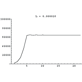
| Say we start with two thousand bunnies, and that the constant L is 0.000028. Then it is simple to calculate that the next generation will have 0.000028 * 2000 * (100000 - 2000) = 5488 bunnies. The next generation after that will have 0.000028 * 5488 * (100000 - 5488) = 14523 rabbits, and so on. We can make a graph of the total number of rabbits in the population. We see that there are some initial small oscillations, but eventually the population settles down to a constant value of 64285. |
 |
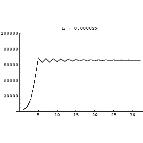
| Say we start with two thousand bunnies,
and that the constant L is 0.000029. We see that there are some
initial somewhat larger oscillations, but eventually the population settles
down to a constant value of 65,517. So increasing L increases the
steady state number of rabbits in the population.
|
 |
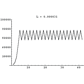
| If we increase the fecundity of the
rabbits by setting L to 0.000031, something very interesting
happens. The population bifurcates and in the "steady state"
oscillates between two different values. Some ecologists now believe that such a "boom-bust" ecological system is better than a stable one. |
 |
| Increasing L to 0.000032 increases the size of the swings in the population. |
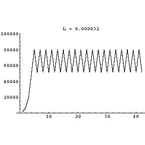 |
| At L equal to 0.000035 the bifurcated population values have bifurcated once again, and the number is now oscillating between four different values! |
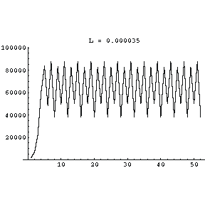 |
| At L equal to 0.0000395 the population values are weird. In fact, the system has now become chaotic. This means that it exhibits all the properties of all chaotic systems. For example, a miniscule change in the initial number of rabbits leads to radical changes in the number of rabbits in each succeeding generation. It also means that the trajectory shown to the right never repeats no matter how many generations we calculate in the graph. |
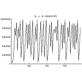 |
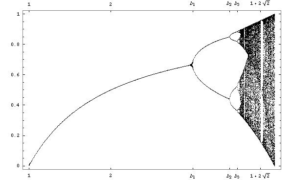
We can calculate the "steady state" values of the population as a function of the fecundity factor L, and the result of such a calculation is above. The graph is called the Logistic Map. We see that initially, as the value of L increases, so does the size of the population. Then we see the first bifurcation of the population, followed by the second, and finally the transition to chaos. There are islands of stability for some higher values of L. We also see a hint in the figure that after the second bifurcation, yet another bifurcation occurs; this in fact occurs. If we zoomed in on the region just before the first transition to chaos, we would see further levels of bifurcation occurring. In fact, it can be shown that these bifurcations occur to an infinite level. This leads us to our next indicator of chaotic systems:
Much of the early work on the logistic equations was done by physicist Mitchell Feigenbaum in the mid-1970's. At this time Feigenbaum's "day job" was at the Los Alamos National Laboratory. He was using the then-new Hewlett-Packard HP-65 hand-held programmable calculator to compute when the next bifurcation in the population would occur as L increased. The HP-65 was wonderful for its day, but now would be considered suitable only for use as a paperweight. It was so slow that Feigenbaum had lots of time on his hands waiting for it to do its calculations. He began trying to guess the value of L for which the next bifurcation would occur.
This led him to discover that the rate at which the bifurcations were occurring was governed by a constant number. If, say, L(n) is the value of L for which the n-th bifurcation occurs, and L(n + 1) is the value where the next bifurcation occurs, then at all levels L(n + 1) divided by L(n) is always the same value. It turns out that this number, now called the Feigenbaum number, is irrational and approximately 4.6692016090... It also turns out that the Feigenbaum number is associated with all chaotic systems.
When one is dealing with circles, it is essentially impossible to avoid having to deal with the irrational number pi, whose value is approximately 3.1415926... This number seems to be intrinsically associated with circular systems and/or the way our minds think about them. Similarly, when one is dealing with systems where the amount of change in some parameter depends on the value of that parameter, the irrational number e keeps showing up in, for example, natural logarithms or exponential growth or decay. So e, whose value is approximately 2.71828..., is somehow associated with these systems and/or the way our minds think about them. These two numbers are pretty mysterious, although many of us have gotten used to dealing with them. Now we seem to have a third such number, this time associated with all chaotic systems: the Feigenbaum number.
The behaviour of the logistic equation is more complex than that of the simple harmonic oscillator. The type of orbit depends on the growth rate parameter, but in a manner that does not lend itself to "less than", "greater than", "equal to" statements. The best way to visualize the behaviour of the orbits as a function of the growth rate is with a bifurcation diagram. Pick a convenient seed value, generate a large number of iterations, discard the first few and plot the rest as a function of the growth factor. For parameter values where the orbit is fixed, the bifurcation diagram will reduce to a single line; for periodic values, a series of lines; and for chaotic values, a grey wash of dots.
Here we describe the most prominent features of this diagram. There are two fixed points for this function: 0 and 1 - 1/r, the former being stable on the interval (-1, +1) and the latter on (1, 3). A stable 2-cycle begins at r = 3 followed by a stable 4-cycle at r = 1 + sqrt(6). The period continues doubling over ever shorter intervals until around r = 3.5699457... where the chaotic regime takes over. Within the chaotic regime there are interspersed various windows with periods other than powers of 2, most notably a large 3-cycle window beginning at r = 1 + sqrt(8). When the growth rate exceeds 4, all orbits zoom to infinity and the modelling aspects of this function become useless.
Bifurcation Diagram of the Logistic Equation

Descriptions of the sort given in the last paragraph are unnatural and clumsy. It would be nice to have a simple measure that could discriminate among the types of orbits in the same manner as the parameters of the harmonic oscillator.
 Consider
two points in a space
X0 & X0 + Dx0
each of which will generate an orbit in that space using some equation or system of equations. These orbits can be thought of as parametric functions of a variable that is something like time. If we use one of the orbits a reference orbit, then the separation between the two orbits will also be a function of time. Because sensitive dependence can arise only in some portions of a system (like the logistic equation), this separation is also a function of the location of the initial value and has the form Dx(X0, t). In a system with attracting fixed points or attracting periodic points, Dx(X0, t) diminishes asymptotically with time. If a system is unstable, like pins balanced on their points, then the orbits diverge exponentially for a while, but eventually settle down. For chaotic points, the function Dx(X0, t) will behave erratically. It is thus useful to study the mean exponential rate of divergence of two initially close orbits using the formula
![]()
This number, called the Lyapunov exponent "l" [lambda], is useful for distinguishing among the various types of orbits. It works for discrete as well as continuous systems.
| l < 0 [lambda] |
The orbit attracts to a stable fixed point or stable
periodic orbit. Negative Lyapunov exponents are characteristic of
dissipative or
non-conservative systems (the damped harmonic oscillator for
instance). Such systems exhibit asymptotic stability;
the more negative the exponent, the greater the stability. Superstable fixed
points and superstable periodic points have a Lyapunov exponent of
|
| l = 0 [lambda] |
The orbit is a neutral fixed point (or an eventually fixed point). A Lyapunov exponent of zero indicates that the system is in some sort of steady state mode. A physical system with this exponent is conservative. Such systems exhibit Lyapunov stability. Take the case of two identical simple harmonic oscillators with different amplitudes. Because the frequency is independent of the amplitude, a phase portrait of the two oscillators would be a pair of concentric circles. The orbits in this situation would maintain a constant separation, like two flecks of dust fixed in place on a rotating record. |
| l > 0 [lambda] |
The orbit is unstable and chaotic. Nearby points, no matter how close, will diverge to any arbitrary separation. All neighborhoods in the phase space will eventually be visited. These points are said to be unstable. For a discrete system, the orbits will look like snow on a television set. This does not preclude any organization as a pattern may emerge. Thus the snow may be a bit lumpy. For a continuous system, the phase space would be a tangled sea of wavy lines like a pot of spaghetti. A physical example can be found in Brownian motion. Although the system is deterministic, there is no order to the orbit that ensues. |
 |
 |
 |
In the diagram below we can see both stable and unstable orbits as exhibited in a discrete dynamical system; the so-called standard map also known as the Cirikov-Taylor map. The closed loops correspond to stable regions with fixed points or fixed periodic points at their centers. The hazy regions are unstable and chaotic.
Sample Orbits of the Standard Map
(x, y) --> (x + y, y - 0.971635 sin (2px)/2p)
Different orbits are assigned different colors.

An interesting diversion. Take any arbitrarily small volume in the phase space of a chaotic system. Adjacent points, no matter how close, will diverge to any arbitrary distance and all points will trace out orbits that eventually visit every region of the space. However, the evolved volume will equal the original volume. Despite their peculiar behaviour, chaotic systems are conservative. Volume is preserved, but shape is not. Does this also imply that topological properties will remain unchanged? Will the volume send forth connected pseudopodia and evolve like an amoeba, atomize like the liquid ejected from a perfume bottle, or foam up like a piece of Swiss cheese and grow ever more porous? My feeling is that the topology will remain unchanged. The original volume will repeatedly fold in on itself until it acquires a form with infinite crenulated detail. End of diversion.
Given this new measure, let's apply it to the logistic equation and see if it works. The limit form of the equation is a little too abstract for my skill level. Luckily an approximation exists. The Lyapunov exponent can also be found using the formula
![]()
which in the case of the logistic function becomes
![]() where
where ![]()
This number can be calculated using a programmable calculator to a reasonable degree of accuracy by choosing a suitably large "N". I calculated some Lyapunov exponents on a programmable calculator for interesting points on the bifurcation diagram. The results are listed in the table below and agree with the orbits.
| r | l [lambda] | comments |
|---|---|---|
| 1 | 0-0.005112... | start stable fixed point |
| 1.99 | 0-6.643... | |
| 1.999 | 0-9.965... | |
| 2 | calculator error* | superstable fixed point |
| 2.001 | 0-9.965... | |
| 2.01 | 0-6.643... | |
| 3 | 0-0.003518... | start stable 2-cycle |
| 3.236067977... | -19.43...* | superstable 2-cycle (1 + sqrt(5)) |
| 3.449489743... | 0-0.003150... | start stable 4-cycle (1 + sqrt(6)) |
| 3.5699456720 | 0-0.002093... | start of chaos |
| 3.56994571869 | 0+0.001934... | start of chaos |
| 3.828427125... | 0-0.003860... | start stable 3-cycle (1 + sqrt(8)) |
| 3.9 | 0+0.7095... | back into chaos |
| 4 | 0+2 | end of chaos |
| *Analytically, |
||
You can see there was some disagreement in the sources as to exactly where the chaotic regime begins. Note also that because the calculator can only approximate the value of 1 + sqrt(5), the Lyapunov exponent for the superstable 2-cycle is only a relatively large negative number and not negative infinity as expected.
The 3-body problem